Introduction
The latest (3rd) edition of Advanced Excel
A textbook for a course in scientific data analysis
A demo of what you can now do in Excel with Matrix and XN
Incorporating Matrix and/or XN functions and macros in VBA
Other features on this website
Problems using the MacroBundle in Excel 2010
An improved macro for the first derivative
Quasi-contour diagrams
Additional aspects of surface graphs
The color index
Excel & VBA pitfalls
Increasing computational precision
The contents of the MacroBundle
The contents of the other downloads
The GNU General Public License
The latest updates
The downloadsThis website is meant for scientists and engineers who want to use the ubiquity, convenience and power of Excel, including its flexibility to go beyond the functionality already provided by Microsoft. It contains freely downloadable, open-access add-in functions and macros for Excel described and illustrated in my book, Advanced Excel for scientific data analysis, 3rd ed., Atlantic Academic 2012, as well as additional information and updates that require color, or arrived too late to be incorporated in the printed version of my book.
You are of course welcome to browse. However, if all you want is to see the SampleSections in order to find out what my book is all about, or whether it suits your needs, just click on Downloads. then select SampleSections1 for the table of contents and selected, complete sections from the first four chapters, SampleSections2 for entire sections from the remaining eleven chapters, and/or SampleSections3 for Appendices C and D and the subject index, where Appendix C lists all functions and macros of Matrix.xla(m), and Appendix D does the same for XN.xla(m). If you want the freely downloadable functions and macros, such as IsoL, the MacroBundle, the MacroMorsels, Matrix, Optimiz, RandomPlot, XN, or any of the other routines used in my book, again select the downloads, and click on the one(s) you want. They are all free for the taking and using!
If you first want to get an idea of what's in these downloads, click on their contents listings, starting with the Contents of the MacroBundle. The downloadable macros and functions are all in open-access VBA source code, and can therefore be modified to suit your individual needs. Most of them are self-documented (mine) or, better yet, come with extensive documentation files (Volpi's). In my book you will find many of them discussed and illustrated, but you do not have to buy my book to use them. What, then, is in my book, so that you might still want to read it?
If I give you a hammer, a screwdriver, a level, a saw, a planer, a chisel, and a few more such tools, will that make you a fine carpenter? Most likely you will still need to learn how and when to use what tool. You can either apprentice yourself to a craftsman, or work through (and especially practice with) a good do-it-yourself book. That is what my Advanced Excel attemps to be. It can also be used as the basis for an introductory (senior undergraduate / junior graduate) course in scientific data analysis, exploiting the fact that many science students prefer the highly visual spreadsheet they are already familiar with to a computer language based on command lines.
Here is what you can expect in my book: descriptions and illustrations, the latter often taken from the scientific literature, of how to select and use a particular method, how and why it works, what its limitations are, and what alternatives are available. The book is really about how to approach and solve scientific data analysis problems, and Excel is used as a widely available, readily learned, powerful and flexible tool to illustrate and implement this. In doing so you become aware of its strengths as well as its weaknesses, extending the traditional boundaries of Excel, and empowering you to do more with it. On the other hand, you will not find fill-in-the-blanks templates, screenshots of Excel dialog boxes, or a rehash of the Excel instruction set. And don't take my word for it, but judge for yourself, by looking at the attached, 3-part SampleSections. They cover more than 16% of my book, and will give you a fair impression of its level and style.
But first the compulsory disclaimer. While I try to make sure that the information provided in this website is correct, and that the downloadable add-in macros and functions work properly, the contents of this website are provided as my opinion, and the downloads are offered "as is", without any warranty. Users of information and/or downloadable material on this website implicitly agree to do so at their own risk and responsibility. And, always, test before trust.
For questions, comments, and suggestions please contact me at
rdelevie@bowdoin.eduIf you want to return to my regular, academic web page, click on
www.bowdoin.edu/~rdelevie/.Click here to advance to the Downloads.
The latest, 3rd edition of Advanced Excel
The third, 2012 edition of my Advanced Excel for scientific data analysis, published by Atlantic Academic LLC, is available only from Amazon.com, still at its introductory price 25% below its list price, or at an even steeper discount of 40% for boxes of 10 books, which makes it more affordable for course work. While its structure has not changed from the second edition (which was published by Oxford University Press), its page size has (from 6" by 9¼" to 8½" by 11") so that the book could include more material without bursting at its spine. It now contains several additional visual tools, and has an even stronger focus on convenience, precision and accuracy. In this new edition you will find many new functions, with explicit examples and applications, especially for using matrix algebra and extended precision software. It contains much new material that you will not find in any other Excel book. The additional material mostly falls in the following categories.
(1) Visual aids. The spreadsheet lends itself eminently to graphically visualizing the essence of least squares, viz. for finding the location of the minimum of a function, using a given criterion. Lars Sillen already introduced a "pit plot" to display log(SSR), the logarithm of the Sum of Squares of the Residuals, as a function of one or two parameters, and this approach is readily implemented with Excel's surface plots or with the Mapper macro from my MacroBundle. The shapes of these plots often alert us to potential difficulties in the least squares analysis, such as significant covariances between various output parameters.
(2) Matrix algebra. The rectangular array of spreadsheet cells makes it a natural medium for matrix algebra, displaying all its elements rather than treating matrices as abstract quantities. Chapter 10 was therefore expanded by emphasizing the convenience and immediacy of the many additional functions of Matrix.xla(m) in, e.g., eigenvalue and eigenvector analysis, and singular value decomposition, including its use for rank reduction in chemometrics.
(3) Extended precision. The power of Volpi's XNumbers has been expanded greatly by John Beyers, who has made it suitable for use on spreadsheets as well as in custom functions and macros. Moreover, the nomenclature used in the newly renamed XN now closely matches that of Matrix, thereby facilitating extended-precision matrix operations on the spreadsheet. Major parts of chapters 10 and 11 were rewritten to accomodate these changes, and to illustrate when extended precision is necessary to obtain reliable answers.
(4) Optimizing. Many scientific and engineering problems involve finding maxima, minima, or zero crossings (roots) of functions. In Optimiz you will find a collection of such procedures, in convenient, directly applicable form. And they are not only handy, but also good: the Levenberg-Marquardt routine in Optimiz, e.g., runs circles around Excel's Solver in any one of the 27 NIST StRD test sets for non-linear least squares analysis. Moreover, as with Matrix and XN, it comes with an extended, very explicit manual full of worked-out examples.
My book, Advanced Excel for scientific data analysis, primarily teaches by example, wherever possible using actual experimental data from the literature, with worked-out exercises and their explicit solutions. It does include explanations of the concepts involved, but these explanations are kept as simple as possible, use a minimum of math, and always leave out any proofs.
Please email me your questions, comments, and suggestions at rdelevie@bowdoin.edu.
Click here to return to the Contents or to advance to the Downloads.
A textbook for a course on scientific data analysis
My book can be used for self-study, as can most Excel books for scientists and engineers. But because of its breadth and depth of coverage, and its wide range of fully worked-out sample problems from the scientific literature, it is also eminently useful for a course in scientific data analysis.
Scientists and engineers now have available a wide range of methods, from least squares to Fourier transformation to digital simulation, from calculus to matrix algebra, from simple graphs to three-dimensional imaging. These are used by physicists, chemists, biologists, geologists, and engineers, and are therefore of interest to a wide range of students and professionals in the “hard” or “physical” sciences. But could you use Excel for such a course?
The answer is “no” if you restrict yourself to what Microsoft provides, simply because Microsoft has targeted its main spreadsheet towards the business community. But it is “yes” once you include a large number of free, open-access add-ins, which extend Excel’s capabilities in many areas of data analysis by providing auxiliary functionality. My book is unique in that it describes many statistical macros that allow, e.g., weighted or moving least squares, provide error estimates to the results of Solver and gives a Levenberg-Marquard alternative, has a Gabor transform algorithm and several macros for deconvolution, highlights an efficient Runge-Kutta function and greatly expanded matrix capabilities, including eigenfunctions and eigenvectors as well as singular value decomposition, and extends the numerical precision from 15 to over 32,000 decimals. Some of it is my own contribution, but most was contributed by an Italian engineer, the late Leonardo Volpi and his many coworkers, and has been extended further by an American computer scientist, John Beyers. Theirs are giant contributions.
But none of that will overwhelm the reader, because the emphasis in my book is on their applications: when and how best to use a given method, what its limitations are, how diverse methods can be combined to get the best of their respective contributions. In many cases, the user will hardly be aware of the distinction between Microsoft’s own functions and macros, and those from its add-ins, because the latter merge effortlessly within Excel’s framework.
In math departments, the course emphasis tends to be on propositions, lemmas, theorems and proofs rather than on practical applications; in a computer science environment it would be on algorithms and writing code; in a statistics department it might be based on a specialized software package with a steep learning curve, such as SAS; and in engineering it would most likely use Matlab. All of these require line-code. By contrast, my book is focused on the data in “data analysis”: the spreadsheet displays all intermediary and final results, and allows you to look at the data and the questions you would like to be solved. And you can choose from a wide variety of methods, and apply them in a visually transparent way.
Such a course can be taught without any mathematical proofs, and without any code-writing, two of the most-dreaded aspects of data analysis for many students, even in the 'hard' sciences. Instead, it uses the world’s most ubiquitous numerical software, with which most students are already familiar from their high school days, and which they most likely already have on their laptops. But for those interested in the background, it gives the essential background information and equations (almost all without their derivations), and provides references to the general literature in each specific area as well as to the sources of its data. And for those so inclined, my book has an extensive chapter on how to write one’s own functions and macros in Excel. Moreover, everything done in background is in fully transparent, open-access code.
In short, you can now teach a course on scientific data analysis using software based on what, with these add-ins, has become a very powerful numerical software package, yet one that most students already have and know how to use. All this with the lowest possible entrance barrier, and with no additional software costs, because the add-ins are all freely downloadable from this website, without the need to buy any additional software, and without any licence fees. A possible outline for such a course at the undergraduate / graduate level is described in the downloads under Suggestions for a data analysis course.
Click here to return to the Contents or to advance to the Downloads.
A demo of what you can now do in Excel
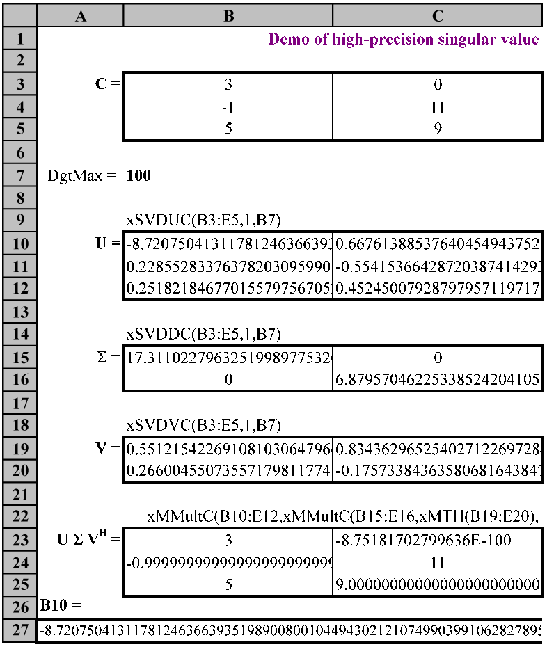
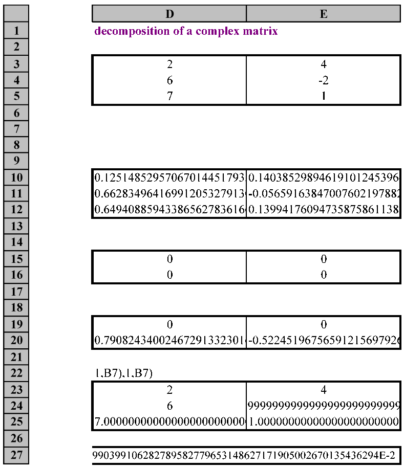
Here is a demo of the type of routine described in the third edition of my book, thanks to the work of Leonardo Volpi, who started writing the add-in programs Matrix and XNumbers, and that of John Beyers, who has now taken over their further development, and contributed the XN routines used below. The demo combines extended precision with matrix algebra far beyond the paltry handful of matrix functions provided by Microsoft. The illustration highlights singular value decomposition (SVD), which is the generalization to rectangular matrices of eigenvalue decomposition, whereas eigenvalue analysis applies only to square matrices. SVD provides the most robust of the available linear least squares methods, and it forms the mathematical basis of many recent chemometric methods, such as principal component analysis, partial least squares, canonical correlation analysis, reduced rank regression, factor analysis, etc.So here is good old Excel, doing singular value decomposition of a complex rectangular matrix at high precision (higher than you are likely to need, now or in the forseeable future), yet with the convenience, transparency, and simplicity of the spreadsheet. No special code to learn; what you see is what you get; and the Paste Function dialog box displays the instruction names and shows you their required and optional arguments, in their proper order. Merely highlight the cell block where you want to see the result, select the appropriate function, and provide it with the necessary input information, just as with any other Excel array function. The example shown here was computed on Excel 2003 running under Windows XP with XN.xla version 6055A; for Excel 2007 and 2010 use XN.xlam version 6055M instead. Of course, as John Beyers keeps improving and extending XN, its version number is subject to change.
a
b
The left-hand (a) and right-hand (b) parts of a single sample spreadsheet illustrating the use of XN instructions for singular value decomposition of a complex, rectangular matrix at 100-decimal numerical precision. Just compare this example with the standard Excel fare, which does not even have any functions for eigenvalue analysis of a square matrix with real elements in regular 15-decimal precision, not to speak of SVD of a complex non-square matrix at high precision. The instruction names can be "read" as follows: the prefix x specifies extended precision, here defined in the argument as the number specified in cell B7; SVD refers to Singular Value Decomposition; U, D (or S, because it contains the singular values si ), and V are the three matrices of the SVD. C signifies that the matrices are Complex; MT specifies a Matrix Transpose, and the superscript H that it is a Hermitean (conjugate, adjoint) transpose, while the prefix x in all these instructions stands for extended precision. The entries in cells B10 and E11 have the multiplier E-2, the other numbers are correct as shown, though only their most significant digits are displayed. All function instructions used, without their = signs, are shown above their cell blocks.
Let me first explain what you see. The top block, in cells B3:E5, here (for the sake of readability) shown in two panels (because the columns are much wider than usual to show more digits) is a complex 3 x 2 matrix labeled C, split into two adjacent blocks, B3:C5 for its real matrix elements in panel a, and D3:E5 for its imaginary elements in panel b. The singular value decomposition then provides its three components, here labeled U, D (or S), and V respectively, where D is the Diagonal matrix containing the singular values in decreasing order of magnitude. For your convenience, the functions used are shown above their matrix cell-blocks (but without their = signs, which would otherwise trigger their implementation). Finally, in order to check that we can indeed recover the original matrix C from this decomposition, we compute the matrix product U D VH, where the superscript H identifies the Hermitean transpose of V.
Because these SVD instructions are functions, they update automatically and virtually instantaneously when you introduce different input data and/or change their computational precision. Even though for this matrix it was pure overkill, a relative precision of 100 decimals was specified, merely to illustrate how easily it is controlled, either by specifying a common value in cell B7, or in the individual instructions by replacing the address B7 by another address or, even more directly, by its desired value. The boxes and labels were added separately, using the standard Excel tools.
The spreadsheet computes or recalculates (when you introduce different input data and/or change its computational precision) to 100 decimal precision (the value 100 is here specified by cell B7), and operates virtually instantaneously on my ten-year-old Dell computer. The spreadsheet shows a small, complex rectangular matrix C in split format, i.e., with its real and imaginary components in side-by-side blocks, in B3:C5 and D3:E5 respectively. (Two other formats, including Excel’s way to cram both real and imaginary components into a single cell, are also supported, and can be selected with 2 or 3 instead of 1 as the last argument. The default is the split format shown here, which is used throughout my book.) In order to show the extended precision and still keep the individual digits readable, the screen is reproduced here in two separate sections, one showing columns A:C, the other columns D:E. Where a single number is broken up in two parts, as in row 27, there is some overlap, an artifact from converting from Excel to a .GIF image.
Cell blocks B10:E12, B15:E16, and B19:E20 show the three components U, D (or S), and V of the singular value decomposition of the complex rectangular matrix C as C = U D VH , where D (or S) is the Diagonal matrix containing the singular values si in decreasing order of magnitude, and the superscript H on V denotes the conjugate (Hermitean, or adjoint) transpose. That the product of these three matrices will indeed reconstruct C is illustrated in cells B23:E25, which (when left-aligned) show the leading digits of the answer, which is here computed to the 100 decimals specified in cell B7. When you use a precision of 50 or 100 decimals, good enough for most problems, the response is virtually instantaneous, but you have access to a numerical precision of up to 32,760 decimals at reduced computational speed. The NIST StRD data often used to calibrate least squares programs used MPFUN, the Fortran predecessor of XN with 500-decimal precision, and then rounded these to 15 or less. So, by comparison, you still have some spare precision over the original NIST test data, by a factor of 65!
The number of decimals displayed is determined by the widths of columns B through E and the font type and size used. Their display stops automatically at a cell boundary with a non-empty cell. Overflow into the empty column F of the above demo was prevented by placing single apostrophes (which do not show) in cells F10:F25; any other (showing) symbol, such as a period, letter(s), number(s), etc. would do as well. The relative computational error is typically less than 1 in 1E-98, i.e., all digits except the last one are usually computed correctly, except when you go full-out in precision, well beyond 32 K.
By left-aligning we here show the first few digits of all matrix elements; the full display of the contents of, e.g., cell C25 would show a nine, a decimal point, followed by 98 zeroes and, at the very end, as the 100th digit, a 9, because the calculated number has an absolute error of 1E-99, but be prepared for these full-precision displays to take up quite a few standard-width columns; in cells A27:E27 their widths have been increased to show the number in cell B10 in its full 100-digit glory. A similar examination of the value in cell B24 with, e.g., the instruction =B24 in an empty spreadsheet cell, say cell B27, will show a minus sign, a zero, a comma, 98 nines, and a 7, because the absolute error is now 3E-99. Note that these numbers are left-aligned, and therefore will not show any exponentials; by making them right-aligned, you can see their tail ends. And to see them in their entirety, either display them on the spreadsheet (as in row of the demo) or, for computations in VBA, in the Immediate Window, or in a Message Box.
You should perform all your computations at the chosen precision. Once you have obtained your final result, you may want to convert that final answer back to double precision with the instruction =xCDbl() before displaying it, but that conversion deletes the extra precision, and should therefore be avoided with intermediate data or when you anticipate having to extend the calculation later.
Few users will need that kind of numerical precision; up to 50 or, at most, 100 decimals is where the most useful improvements are found. For simple cases I usually set the number D of decimals used to 35, then see whether the answer changes in its 15th decimal with D = 50. If not, I tend to trust the results, otherwise I go to D = 100. There is of course a speed penalty for very large numerical precision, as specified below.
The input numbers in C (in block B3:E5) are not restricted to integer values; these are used here only so that the answers in B23:E25 are more easily interpreted. My book describes how, where, and why SVD is used, and shows several detailed examples.
The SVD algorithms used here are not new, but thanks to John Beyers this type of advanced computer math is now available in the convenient and ubiquitous Excel format. The equivalent routines (and many more) are also available in double precision. If you don't need extended precision, merely delete the prefix x from the instructions and the (optional) reference to DgtMax in their arguments, and make sure that Matrix.xla(m) is loaded and installed also; the two will happily coexist in your spreadsheet.
A note for connoisseurs: these functions use the “compact” SVD formalism, in which U is m´n, D is n´n, and V is n´n, when C is m´n. For the more symmetrical, “full” format, in which U is m´m and D is m´n, just add the requisite number of zero elements. The functions do not require that m ³ n; when m < n, the compact formalism yields U as m´m, D as m´n, and V as n´n.
What does this calculation take? All of the Excel instructions used are shown here, only functions are used (i.e., no macros are involved), nothing is done and/or hidden in background. (Even the functions themselves, unlike Excel's, are open-access, although you will need to know something about VBA and about modular coding to be able to "read" their code.) The commands used are block instructions, because that is how Excel deals with matrices, i.e., the appropriately sized blocks are highlighted before you type the command, the instruction is typed, and then entered with the block enter command CtrlÈShiftÈEnter. And you must have XN.xla or XN.xlam loaded onto your machine and incorporated in your Excel.
Note: when downloading XN.xlam6055M.zip push the “Office Button” in Excel 2007, or the “File” tab in Excel 2010, check under Excel > Options > Formulas > Calculation Options and, if necessary, set these to Automatic. Make sure to read the included help file XN.chm in order to use the correct configuration settings, to handle the Windows security measures, and for general information.XN is freely downloadable software, without ads or other garbage. You select its precision, within the limit determined by the version loaded; the maximum precision available is now 32,760. You need to download only one routine, either XN.xla60xx for Excel95/2000/XN/2003 or XN.xlam60xx for Excel2007/2010, where xx denotes the version. Each version uses a Maximum Digits Limit of either 816 or 32,760, which you select in the XN toolbar > X-Edit > Configuration, and then fix by pushing Set. You then select the value of D within the chosen range; you can still use another D-value within that range for each particular function.
So much new (and, I hope, interesting and useful) material was added that it took me much longer than I had anticipated to finish this third edition. Fortunately, it is now available from Amazon. Look under "Advanced Excel for scientific data analysis" for its large, brightly colored cover, and especially for the specification "3rd edition".
Few scientists will need more than 816-decimal precision, but some mathematicians may. At any rate, it is nice to have that power at your fingertips in case you need it. But how fast is XN? Since it performs all of its operations in software, i.e., by bypassing the speed-optimized numerical hardware of the cpu, it is bound to extract a premium in terms of execution time, and it does. How much depends, of course, on the computer you use; if you want to know, use the function xTimingMult shown below for multiplication, and/or modify it for whatever mathematical operation other than multiplication you want to speed-test. Use a sufficiently large number i of repeats, say 10,000 or more, to get a reasonable estimate. You can also modify the function to test Excel's native routines, and then compute the factor by which XN slows you down.
Function xTimingMult(i, D)
' a VBA test function to estimate the
' time for i repeat multiplications at
' an extended precision of D decimalsDim e, p, Time1, Time2, xSum, xProduct
Dim j As Long, ii As Long
ii = i
Interval = 0
xSum = 0
p = xPi(D)
e = xE(D)
Time1 = Timer
For j = 1 To ii
xProduct = xMult(p, e, D)
xSum = xAdd(xSum, xProduct, D)
Next j
Time2 = Timer
xTimingMult = Time2 - Time1
Debug.Print "D = " & D & ": Time taken = " _
& Time2 - Time1 & " for " & ii & " repeats."
Debug.Print "p = " & p
Debug.Print "e = " & e
Debug.Print "xSum = " & xSum
Debug.Print ""
End FunctionClick here to return to the Contents or to advance to the Downloads.
Incorporating Matrix, Optimiz, XN etc. in VBA
The above example illustrated a direct use of Matrix and XN in the spreadsheet. Here is an illustration of the ease of introducing Matrix into VBA code; the situation with XN is no different. The example given below addresses the need of many chemometric methods (such as factor analysis, principal component analysis, partial least squares, and canonical correlation analysis) to reduce the rank of a matrix. This comes up, e.g., when there are many (perhaps insignificant and/or mutually dependent) variables, and one wants to use only the dominant variables, often called "factors" or "princial components". The function code shown below reduces the matrix rank by one, and can of course be used repeatedly to reduce the matrix rank further. The main point of this example is to show how easily Matrix.xla(m) integrates with VBA; the same applies to XN.xla(m).
Here, then, is the code, followed by a brief explanation, and some numerical examples. As you will see, once you have installed Matrix.xla(m) and/or XN.xla(m) in Excel, the spreadsheet treats these add-in functions and macros as its own. Moreover, after you also (separately) introduce Matrix.xla(m) and/or XN.xla(m) into VBA, you can incorporate them effortlessly into your own custom functions and/or macros.
The Matrix functions used here are SVDU, SVDD, and SVDV, which yield the three matrix components of the singular value decomposition of a rectangular matrix R, and the convenient Matrix function MProd(S1, S2, S3, ...), where S denotes a square matrix
Function RankReducer(R)' Select a block that has as many rows as R, but one fewer column.
' Then, when the matrix R is nR by nC+1, the output will be nR by nC.Dim i As Long, j As Long, nC As Long, nR As Long
Dim DArray As Variant, DDArray As Variant, RArray As Variant
Dim UUArray As Variant, VTArray As Variant, VVTArray As Variant' Copy R to RArray:
RArray = R
' Determine the dimensions of R:
nR = UBound(RArray, 1)
nC = UBound(RArray, 2) - 1' Redimension the arrays now that nC and nR are known:
ReDim DDArray(1 To nC, 1 To nC) As Double
ReDim VVTArray(1 To nC, 1 To nC) As Double'Use the singular value decomposition functions:
DArray = SVDD(RArray)
UUArray = SVDU(RArray)
ReDim Preserve UUArray(1 To nR, 1 To nC)
VTArray = MT(SVDV(RArray))For i = 1 To nC
mmFor j = 1 To nC
mmmmVVTArray(i, j) = VTArray(i, j)
mmmmDDArray(i, j) = DArray(i, j)
mmNext j
Next i' Output the rank-reduced matrix RR:
RankReducer = MProd(UUArray, DDArray, VVTArray)
End Function
The principle of the method is as follows. The minimally invasive way (optimal in a least-squares sense, i.e., in terms of its Frobenius norm) to reduce the number of independent variables of a matrix (with possibly redundant columns) by one is by using instead a matrix in which the smallest singular value is neglected. To do so we take a rectangular matrix R, determine its number of rows and columns, and compute its singular value decomposition, R = U D VT. We delete from U its right-most column, and from D and V their bottom row and right-most column, and reconstitute the rank-reduced matrix by using RR = UU DD VVT with the now modified UU, DD, and VV.
Here is an example. Say that you have the rectangular matrix R in B3:D7, and want its rank reduced. Highlight a block that is one column narrower than R, such as F3:G7, call RankReducer, and block-enter it. Done!
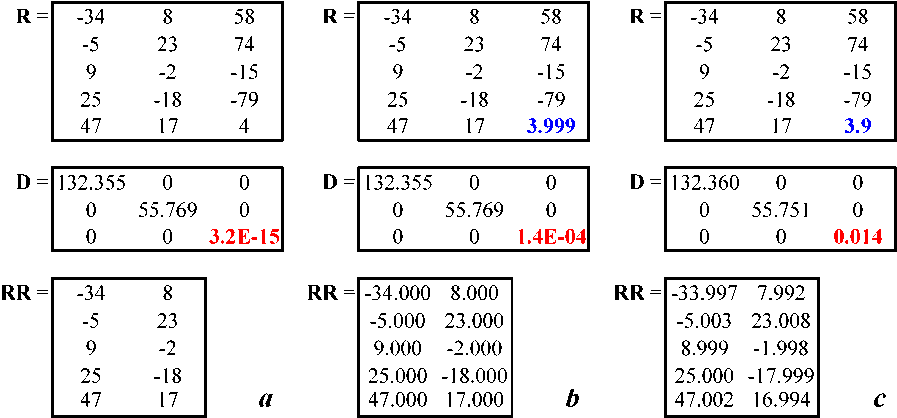
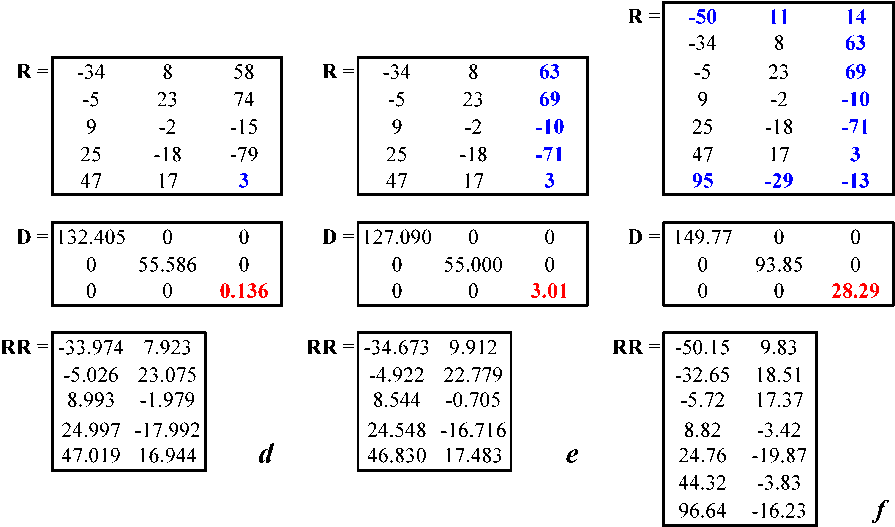
There is also a corresponding macro, ReduceRank(), which performs the same function but also shows you the singular values, with its smallest (to be deleted) value highlighted in bold red. The macro then asks you whether or not to proceed with the rank reduction, something a function cannot do. The following samples show the macro output. The function merely shows the rank-reduced matrix, but neither displays the singular values nor asks you whether you want to go on with the rank reduction.
The first example, a, is of a matrix R that is singular, since the first column minus three times the second equals the third. The smallest singular value therefore ought to be zero, but isn't quite because of computer round-off. But when that singular value is removed, the first two columns of R are reproduced intact.
When one or more elements of R are changed slightly (as highlighted in bold blue), the resulting rank-reduced matrix is still quite similar to its original, but as we change R further away from a singular matrix, as in b through f, the smallest singular value becomes less and less neglegible versus its next-smallest neighbor on the diagonal of D, and the resulting distortion due to rank reduction increases. That is the trade-off.
The (initially singular) input matrix R, the corresponding matrix D with its singular values, and the rank-reduced matrix RR, as R increasingly moves away from singularity from panel a to panel f. Each panel shows three matrices, R, D, and RR, one below the other.
For a specific example of modifying an Excel macro to higher numerical precision by incorporating XNxla(m), see my xnLS linear least squares macros, which are modified from the LS macros in my MacroBundle, as specified on pp. 568-578 of the latest edition of my Advanced Excel book, where the modifications are highlighted in bold printing.
These modifications are relatively few, but the result is stunning: with a numerical precision of 35 or more decimals, xnLS nails all coefficients and standard deviations of the entire collection of NIST StRD linear least squares test data sets, including their last digits. This illustrates (1) that such modifications are quite straightforward, (2) that you don't need a very sophisticated least squares routine, because the numerical precision is usually the limiting factor, and also (3) that you usually do not need to go to very high data precisions to get your answers right: in this case you need only 35 of the available 32,760 decimals!
Click here to return to the Contents or to advance to the Downloads.
Other features of this website
Many topics discussed on the website of the second edition of Advanced Excel are now included in its third edition and/or in the MacroMorsels, and therefore no longer need to be displayed here. Two items that have been retained here are the notes on the color index, because black printing ink has difficulty conveying color, and the description of extended macro precision, because you might not otherwise know that it is now possible in Excel to compute with up to more than 32 K decimals. As before, new developments that came too late to be included in the latest printed edition will be added here. The number of downloadable files has increased. You will find an enlarged set of macros in the MacroBundle, many of which are also improved through the use of color-coded outputs and/or self-documenting cell comments. The new macros include those for integration and differentiation.
The collection of MacroMorsels has also grown, and readers are cordially invited to suggest further additions or, better yet, to submit them. All of my downloadable .doc files are copyrighted under the GNU General Public License to guarantee that you can freely download, use, share, and modify this software, without risk that it will be hijacked for commercial and/or promotional use.You may want to save and/or print the downloaded files before installing the .doc files in your Excel VBEditor module. If you dislike any of them, please let me know why, and preferably suggest ways to improve them. On the other hand, if you like them, spread the word, and if you use them in a publication, please refer to their source, i.e., to this website and/or to the book. In addition to the above, this website now also contains several additional, freely downlodable software packages, almost all with open access to their code.
XN.xla(m) has now replaced Xnumbers.dll, but the latter is still available for downloading. Users of Excel 2007/2010 may experience difficulties loading Xnumbers.dll because of problems with Microsoft's reg files. A possible remedy is described at the end of the section describing the xMacroBundle. However, because XN is much more powerful and much more convenient, I suggest that you convert any XNumbers files you may still have to XN. Moreover, the conversion from XNumbers to XN is quite easy.
Click here to return to the Contents or to advance to the Downloads.
Problems using the MacroBundle in Excel 2010
Some users of Excel 2010 may experience problems with macros with names that could be misread as cell addresses, specifically LS1, ELS1 and WLS1, because Excel 2010 can misinterpret those macro names as cell addresses, even in the absence of a leading equal sign. (Excel2007 did not have this problem, and Excel 2010 shouldn't have had it either .) A give-away was that LS0, ELS0 and WLS0 do not give such problems, because Excel's row numbering starts with row 1, so that the number 0 cannot be misread as part of a cell address.
The names were originally coined because LS0 uses no intercept, while LS1 uses one, and the typographically similar all-letter names LSO and LSI (for Least Squares through the Origin and Least Squares with an Intercept respectively) will simply avoid this problem. These changes have now been incorporated in the latest version of the MacroBundle, which you can download below. I thank Lena Jankowiak and Prof. Tiny van Boekel of Wageningen University in the Netherlands for bringing this problem and its solution to my attention.
An improved macro for the first derivative
An improved double-precision macro, Deriv1, for numerically computing the first derivative df(x)/dx of a given function f(x) at a specified value x was written, and is now incorporated in the MacroBundle, as well as its extended-numberlength version xnDeriv1 in the xnMacroBundle. (Note that this, in fact, yields a partial derivative.) The theoretical basis for this improved algorithm nicely illustrates the interplay between inaccuracy and imprecision in numerical analysis, and is described in chapter 9 of my book, see in SampleSections2 under sections 9.2.9 and 9.2.10). It can also be found in J. Chem. Sci. 121 (2009) 935-950, freely accessible at http://www.ias.ac.in/chem.sci/Pdf-Sep2009/935.pdf. The macro uses central differencing, and allows the user to select the number j of equidistant data points of the function to be sampled, where j is an odd positive number between 3 and 15. The achievable accuracy depends, of course, on the specific function f(x) and on the particular value of the argument x at which the derivative is computed, but the macro often yields answers with at least 9 (and often 10) significant figures for j = 3, 11 significant decimals for j = 5, 12 for j = 7, and 13 for j = 9 or higher.
In double-precision arithmetic there is little advantage in going to j-values beyond 9, because cancellation noise may then limit the resulting accuracy; on the other hand, there is the real disadvantage of the larger footprint at higher j-values, which increases the chance of invalidating the answer by reaching across a nearby discontinuity or singularity.
Moreover, keep in mind that all such problems of limited accuracy and large footprints disappear when extended-precision software is used. Likewise, extended pecision obviates the need for analytical derivatives in optimization routines such as the Levenberg-Marquardt algorithm.
Click here to return to the Contents or to advance to the Downloads.
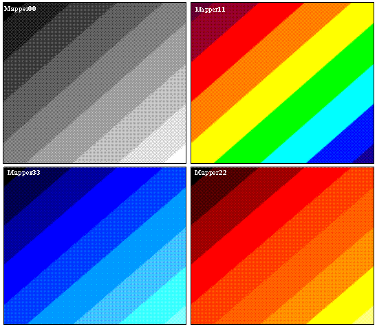
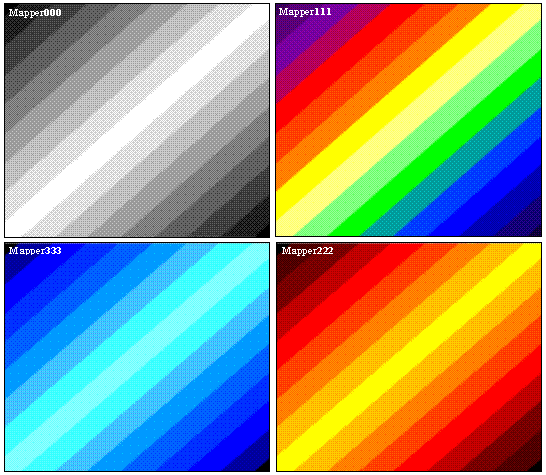
The set of available Mapper macros has been extended to provide two extra types of quasi-contour diagrams. They use stepwise rather than continuous color changes, and therefore display color bands. For a sufficiently large array, of at least 100 by 100 cells, they are considerably faster to make (because they do not require any additional interpolations) than IsoL.xla, and approach a similar visual resolution. For smaller arrays, pixellation will show as serrated edges where IsoL.xla still exhibits clean curves. Samples of these Mapper macros are shown here for a simple 150 by 150 cell test array with gradually increasing numerical values from the top left to the bottom right. The first number n in the names of these routines follows the color scheme of Mappern, doubling the number n following the term Mapper to nn yields bands in a single progression, while triple numbers nnn show bands that have maximum brightness in the middle region of the cell values used. Moreover, the old Mapper1 has been modified, and the MBToolbar has been modified to incorporate these new Mapper macros.
Quasi-contour plots for a gradually increasing value, clockwise, for a gray scale (Mapper00), a spectral scale (Mapper11), a red scale (Mapper 22) and a blue scale (Mapper 33).
Quasi-contour plots for a gradually increasing value, clockwise, for a gray scale (Mapper000), a spectral scale (Mapper111), a red scale (Mapper 222) and a blue scale (Mapper 333).
Click here to return to the Contents or to advance to the Downloads.
Additional aspects of surface graphs
Section 1.4 of Advanced Excel 3rd ed. briefly describes 3-D surface graphs. Nenad Jeremic kindly sent me the following information, which I gladly share here.1. When you hold dow the Ctrl key while rotating a 3-D surface graph with your mouse, Excel will continuously plot outlines of the surface. This helps you to fine-tune the effect of rotating the graph.
2. You can add shading to a 3-D chart as follows. After you have made the graph, select a single color in the chart legend box. Right-click on it, select Format Legend Key, go to the Options tab, and select the 3-D shading option check box. The shading will then be applied to all colors, i.e., to the entire graph.
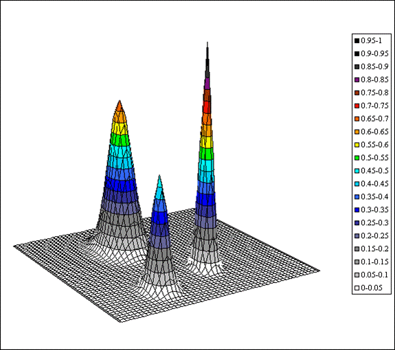
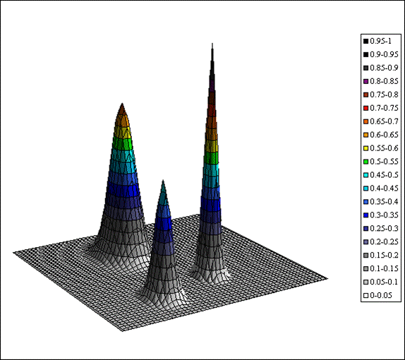
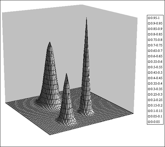
This effect is most useful when the grid lines are fairly widely spaced. If you apply the shading first, and then rotate the graph, the shading also rotates, which can make for a more dramatic effect. The figures illustrate this effect for the three-peak surface diagram of Fig. 1.4.2 in the third edition of my book (AE3) on p. 21. As you can see, it can make these plots more appealing in both color and black & white.
Colored plot, no shading.
Colored plot, with shading.
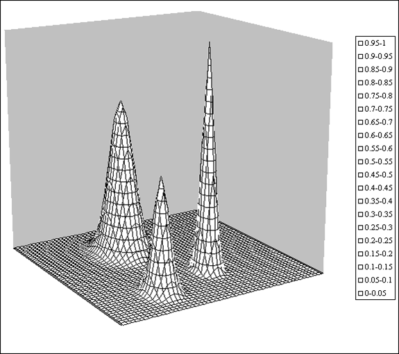
Black & white plot, no shading.
Black & white plot, with shading.
Click here to return to the Contents or to advance to the Downloads.
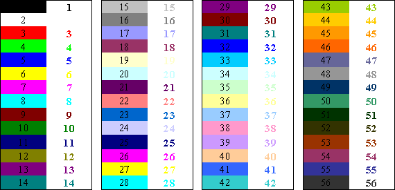
The Microsoft Office suite has two sets of color schemes. The more elaborate one, called RGB, lets the user select mixtures of red, green, and blue. It is used, e.g., in the Mapper macro of the MacroBundle. A simpler, more limited color scheme, based on a small number of color samples, is used by Excel in the FillColor and FontColor icons on its Formatting toolbar. Those (Excel 1997/2000/2003 color swatches have names that show when you hover over them with your mouse, but in order to refer to them in a macro, you need their ColorIndex, an integer. Below you will find these, following the routine used to determine them. Make two adjacent columns of numbers from 1 to 14. and two each of 15 (1) 28, 29 (1) 42, and 43 (1) 56. Highlight the top cell of the first column, containing the number 1. Switch to the VBEditor with either AltÈF11 on a pc, or OptÈF11 on a Mac. (If this is the first macro, open the module by selecting Insert > Module in the Visual Basic Toolbar.) Then write the following macro:
Sub color()
Dim cellValue As Integer
cellValue = Selection.Value
ActiveCell.Interior.ColorIndex = cellValue
Selection.Offset(1, 0).Select
End SubNow hit the F5 key repeatedly, then switch back to the worksheet with AltÈF11 (pc) or OptÈF11 (Mac), and see what happens. Better yet, display the spreadsheet and the macro side-by-side, without overlap, so that you can switch easily between them. (On a narrow monitor you may have to reduce the size of the speadsheet to avoid overlap.) You now should have colored the first cell black, the third red, the next ones bright green, blue, yellow, pink, turquoise, etc. Now repeat this on the third, fifth, and seventh column. Then change the word Interior in the above code into Font, and repeat the above in the even-numbered columns. This is what you should get:
ColorIndex by the numbers, for both Interior and Font.
When you click on the down arrow of Excel's color icon in the Formula bar, and then hover with your pointer over the 40 color swatches shown, you will find their names. Putting the two together yields the following display of color, ColorIndex values, and Microsoft color names:
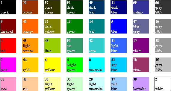
ColorIndices and corresponding Microsoft color names of the samples of FillColor and FontColor.
The above macro indicates how you can manipulate cell and font colors in a macro. (A function cannot do this.) All you need to do is to select an ActiveCell, and then to specify what you want, as in
ActiveCell.Interior.ColorIndex = 8to color the whole cell turquoise, and/or
ActiveCell.Font.ColorIndex = 5
to make its text blue.
Please note that a different set of colors, typically less saturated and with different names, is used in Excel 2007/2010 in the Font section of its Home ribbon. However, the old ColorIndex still works in these newer versions.
Click here to return to the Contents or to advance to the Downloads.
Excel is the most ubiquitous numerical software available, bar none. But that does not mean that it is flawless: popularity is no guarantee for quality. Here are some of its most egregious sources of errors; their order of importance for you depends, of course, on the type of problems you try to solve with it. At any rate: forewarned is forearmed.
1. In Excel, negation comes before exponentiation while, as usual, exponentiation comes before subtraction. Of course, negation and subtraction use the same minus symbol “–”, and because it makes a difference in Excel (whereas it should not), the software guesses from the context what you might mean, and it often guesses wrong. This is one of those places where Excel, in order to make things supposedly easier, actually makes them much worse. To add to the confusion, Excel's customer scripting language VBA doesn’t do this, but always (correctly) exponentiates first. Here is a simple example. Say that you want to use the common central differencing formula for a first derivative,
f I(x) = [f(x+d) – f(x–d)] / (2 d)with x = 1, d = 0.1, and f(x) = x2. If you write =(1.1^2–0.9^2)/(2*0.1) you will find the correct result (1.21 – 0.81) / 0.2 = 0.40 / 0.2 = 2, whereas =(-0.9^2+1.1^2)/(2*0.1) will net you the incorrect answer (+ 0.81 + 1.21) / 0.2 = 2.02 / 0.2 = 10.1. However, when you use either form in a function or macro, i.e., in VBA, the answer always comes out right. So here you have it, in a more obvious form: in Excel, +1.1^2–0.9^2 is not equal to –0.9^2+1.1^2, or + a2 – b2 is not the same as – b2 + a2. And this applies not just to squares, but to all even-integer powers of a and b. Understanding what went wrong suggests the following remedies, which indeed work:(1) Use brackets around a term and its exponent: (a2) – (b2) = – (b2) + (a2), so that you would replace (–0.9^2+1.1^2)/(2*0.1) by =(–(0.9^2)+ (1.1^2))/(2*0.1) or =(–(0.9^2)+ 1.1^2)/(2*0.1); or
(2) Use –1* instead of –, as in a2–1*b2 = –1*b2 + a2, so that the above expression would read (–1*0.9^2+1.1^2)/(2*0.1).
Note that XN avoids this problem altogether, because (1) it uses the very same instructions for the spreadsheet and for its VBA code in functions and macros, and (2) it uses different instructions for negation, =xNeg(a) for –a, and for subtraction, =xSub(b,a) for b–a.
The following two examples are only of concern to those of you who use custom functions and macros, and illustrate mismatches between the spreadsheet and its customer scripting language VBA. You can find more such examples in section 1.14 of Advanced Excel, but you get the idea: test before you trust.
2. In Excel, LOG denotes 10-based logarithm, and LN specifies the natural logarithm, its e-based counterpart. But in VBA, log means natural logarithm, and the 10-based logarithm of the number a must be computed as Log(a)/Log(10), or by referring explicitly to the Excel formula with Application.Log(a).Again, XN avoids this problem: both on the spreadsheet and in its functions and macros it uses =xLog(a,b) for logb(a), =xLog(a) for log10(a), and xLn(a) for loge(a) = ln(a).
3. In Excel, ROUND always rounds away from zero: ROUND(0.5) produces a 1, and ROUND(–0.5) results in –1, whereas VBA rounds to the nearest even integer, so that both Round(0.5) and Round(0.5,0) yield 0, while Round(–0.5) and Round(–0.5, 0) displays –0 or, in scientific notation, as –0.00E–01 with as many decimal places as you care to specify. (This particular result is interesting because, despite the specific inclusion of –0 in the standard IEEE 754 protocol, Excel doesn’t recognize –0, and doesn’t even let you type it in as a number, yet it generates and displays it here!)
XN has three rounding functions: xRound(a,d) rounds a to d decimals behind the decimal point, just like Excel's ROUND(a,d). xRoundR(a,d) rounds relative, i.e., d now specifies all decimals rather than just those behind the decimal point. And the special vRoundR(a,d) finds the banker's relative rounding, with a final 5 rounded to the nearest even digit.
Click here to return to the Contents or to advance to the Downloads.
Increasing computational precision
The macros in the MacroBundle are relatively crude, and contain none of the computational sophistication that you might expect from a professional programmer or applied mathematician, simply because its author is neither. They could certainly be made to be more modular, more efficient, and more accurate. But many scientists and engineers have neither the time nor the expertise to write VBA code that squeezes the last few significant digits out of their macros. This section does not directly address that problem, but offers what may often be an efficient end-run around it.
First a bit of semantics. We will stay with the usual distinction made in the physical sciences between accuracy and precision, with accuracy indicating how closely one approximates the true answer, and precision defining the reproducibility of a given procedure with a given method. Computers are fully deterministic machines, and are therefore (except when they malfunction) precise to within the number of digits displayed in their results. In other words, repeating a computer calculation under identical conditions should yield completely reproducible answers, for whatever they are worth, and its numerical precision should therefore equal its numberlength. For example, Excel shows all of its results in industry-standard double precision, i.e., with 64 bits, corresponding to about 15 decimal places. There is, of course, no guarantee that all (or even any) of the 15 digits in the result of such a computation are numerically accurate. That is why organizations such as NIST publish test sets to calibrate software accuracy.The numerical accuracy of a computer program cannot exceed its numerical precision, but it can be much smaller. Still, in many applications, double precision yields perfectly adequate accuracy.
However, there are also many situations, such as when large matrices must be manipulated, in which the numerical accuracy during data analysis may be degraded sufficiently to cause it to produce answers of dubious usefulness. In those cases it may be necessary to use more precise software. One may not even be aware of this: what fraction of the many users of Excel's Trendline would know that, in fitting their data, Trendline uses matrix algebra? The recently updated and expanded, very powerful XN.xla(m) freeware package of John Beyers, building on the earlier XNumbers.xla of Leonardo Volpi and his team in Italy, has now made it both possible and easy to extend the numberlength limits of Excel macros, and hence their numerical precision, provided that you have access to their code. With this new software addition you can obtain much more accurate results from the spreadsheet, from functions, and from macros, and you can also use XN to test the accuracy of code fragments, i.e., to identify accuracy-limiting code. This freeware, which can be downloaded from this website as well as from its originating website, http://www.thetropicalevents.com/XNumbers60.htm, is a great gift to scientific users of Excel. You will need an unzip routine on your computer.
The approach used in XN is similar to that of MPFUN77 for Fortran 77, see D. H. Bailey, ACM Trans. Math. Software 19 (1993) 288-319, and its current successor, ARPREC (arbitrary precision) for Fortran 90 and C++, see http://crd.lbl.gov/~dhbailey/mpdist/. XN allows Excel versions 2000 through 2010 to make calculations with a user-selectable numberlength of up to 32 K decimal places. If no numberlength is specified, XN will use its default setting of quadruple precision (of about 29 decimals), which is often sufficient. This default value can of course be user-modified; mine is usually set to 35 or, when I anticipate problems, to 50, or even 100. The speed difference between these is usually unnoticeable.
Note that XN works just as well on the spreadsheet as in the VBA code of functions and macros. Moreover, your macros can keep their original input and output formats, so that, to their users, they "look and feel" exactly the same as before, except for their slower execution speed (at very high precisions) and the (often) higher accuracy of the results. Practical examples will soon be put in the xnMacroBundle. The first macro to go into that bundle, xnLS, is described in detail in section 11.14 of the latest (third) edition of my book.
That macro is an example of taking a rather unsophisticated routine, LS, based on simple matrix inversion, that could not even get the first digit right of the NIST linear least squares test Filip, and converts it into a champ, xnLS, that gets all 15 decimals right with D = 35. No need for SVD and proper polynomial averaging! The same applies to differentiation using simple first-order central or lateral differencing: with D = 35 you can use these to get your answers consistently with all correct decimals, and even use smaller excursions into neighboring territory, where discontinuities or singularities may lurk. Crude and unsophisticated, perhaps, but directly addressing the source of the problem, viz. the sometimes insufficient numerical precision of "double" precision.
To get an idea of the range of XN, take a look at Appendix D in the downloadable SampleSections3.
Click here to return to the Contents or to advance to the Downloads.
The contents of the MacroBundle
This is a collection of macros, with many now using self-documenting cell comments. (Eventually all my macros will be so modified, but unfortunately I can find no more than 25 hours in my days.) Further improvements may be inserted, and new macros added, as they become available. The most recent incarnation of the MacroBundle is version 10.The macros in the MacroBundle are all open-access and self-documented, and can be downloaded freely and used without any obligation, as long as they are not used commercially. Because they are distributed as a text file, you can readily inspect them. If you dislike them, please let me know why, and preferably suggest ways to improve them. If you like them, please spread the word, and if you use them in a publication, please refer to their source, i.e., either to this web site or to the book. The more people know about the existence of these free, open-access macros, the more people may benefit from them, which is the purpose of making them freely available in the first place. Disclaimer: the macros in the MacroBundle were created to accompany my two recent books, How to use Excel in Analytical Chemistry and in General Scientific Data Analysis, Cambridge University Press 2001, and its most recent, more general successor, Advanced Excel for Scientific Data Analysis, 3rd ed., Atlantic Academic 2012. They were written primarily to illustrate how to analyze data, and also how to write (relatively simple) macros to achieve that goal when not already available in Excel. These rather unsophisticated macros will usually do what they are supposed to do, but because of their simple input and output formats they are neither made nor meant to be foolproof, and they may not always generate the best possible results either. They are provided free of charge, and without any warranty, implied or otherwise. The same applies to the macros in the xMacroBundle, the MacroMorsels, and the xMacroMorsels. Installation instructions are included in the package, and apply to the individual macros as well as to the total bundle. In order to keep them free of commercial exploitation, they are all copyrighted under the GNU General Public License, details of which you can find in the GNU General Public License download.The direct uses of the macros in the MacroBundle are briefly described below. They can also be used to model your own macros, be modified to suit your individual needs or tastes, or even be scavenged for useful parts.
Propagation of imprecision
Propagation computes the propagation of imprecision for a single function, for various independent input parameters with known standard deviations, or for mutually dependent parameters with a known covariance matrix.
Linear least squares
LS is a traditional least squares fitting routine for linear, polynomial, and multivariate fitting, assuming one dependent variable, and as many independent variables as may fit your fancy. LSO forces the fit through the origin, LSI does not. The output provides the parameter values, their standard deviations, the standard deviation of the fit to the function, the covariance matrix and, optionally, the matrix of linear correlation coefficients.
ELS provides least squares smoothing and differentiation for an equidistant (in the independent variable) but otherwise arbitrary function using a "Savitzky-Golay" moving polynomial fit. ELSfixed uses a user-selected, fixed-order polynomial, ELSauto self-optimizes the order of the fitting polynomial as it crawls along the function. Philip Barak of the University of Wisconsin contributed this macro.
WLS is the equivalent of LS with the inclusion of user-assigned weights.
GradeBySf uses the standard deviation of the fit to a multivariate function of up to six variables as an aid to find the optimum number of such variables.
LSPoly applies LS to fitting data to a polynomial of gradually increasing order (up to 14), including criteria (such as sf and the F-test) useful for deciding how many terms to include in an analysis.
LSMulti applies LS to an increasing number of terms of a multivariate least squares analysis.
LSPermute computes the standard deviation of the fit for all possible permutations of multivariate parameters of up to six terms.Nonlinear least squares
SolverAid provides uncertainty estimates (standard deviations, the covariance matrix, and optionally the matrix of linear correlation coefficients) for Solver-derived parameter values.
SolverScan lets Solver scan a two-dimensional array of parameter values. It requires that Solver.xla is installed.
ColumnSolver applies Solver line-by-line to column-organized data. It requires that Solver.xla is installed.Transforms
FT is a general-purpose Fourier transform macro for forward or inverse Fourier transformation of 2n data where n is an integer larger than 2.
Gabor provides time-frequency analysis.
Ortho yields Gram-Schmidt orthogonalization.(De)convolution
(De)convolve provides convolution and deconvolution. The convolution macro is quite generally applicable, the deconvolution macro is not.
(De)ConvolveFT yields convolution and deconvolution based on Fourier transformation.
DeconvolveIt performs iterative (van Cittert) deconvolution. DeconvolveIt0 has no constraints, DeconvolveIt1 assumes that the function is everywhere non-negative.Calculus
Deriv uses central differencing to find the first derivative of a function.
Deriv1 is a higher-precision version of Deriv.
DerivScan applies Deriv to a range of step sizes.
Romberg efficiently integrates a function.
Trapez uses straightforward trapezoidal integration, useful for repetitive functions.
Semi-integrate & semi-differentiate comprises two small macros for cyclic-voltammetric (de)convolution assuming planar diffusion.Mapper
Mapper generates color (or gray-scale) maps of a rectangular array of equidistantly spaced data. At present it contains 12 specific sample maps, four using a gradual color change, four with nine discrete color bands, and four with 17 such color bands. The four color schemes used are a gray scale, a color spectrum, a predominantly red scale, and a predominantly blue one. Since these are all open-access, you can easily add your own color scheme if you so desire; the process is described in the MacroMorsel WriteYourOwnBitMap.
Miscellany
ScanF generates an array of a function F(x,y) of the two variables x and y for subsequent use by Mapper or, optionally, of an input list for SimonLuca Santoro's IsoL macro for creating contour maps.
RootFinder finds a single real root by bisection.
MovieDemos has the code for the simple examples given in my Advanced Excel book.
InsertMBToolbar provides easy access to the macros of the MacroBundle. Can be used in Excel 2000/2003 and in the Developer ribbon of Excel 2010.
RemoveMBToolbarClick here to return to the Contents or to advance to the Downloads.
The contents of the other downloads
There are three sample sections: SampleSections1 contains the preface, table of contents, and one or more complete sections from each of the first four chapters. SampleSections2 contains one or more complete sections from each of chapters 5 through 11, while SampleSections3 contains appendices C and D in their entirety, as well as the subject index. Because the chapter sections are largely self-contained, these selections from the third edition of my Advanced Excel for Scientific Data Analysis can give you an idea of what to find in my book in terms of contents, type of coverage, and style. Below are the sections shown.
SampleSections1:
Preface
Contents
Chapter 1:
Survey of Excel
Band mapsChapter 2: Simple linear least squares
How precise is the standard deviation?Chapter 3: Further linear least squares
Phantom relationsSpectral mixture analysis
The power of simple statisticsChapter 4: Nonlinear least squares
Titration of an acid salt with a strong baseSampleSections2:
Chapter 5: Fourier transformation
Analysis of the tidesChapter 6: Convolution, deconvolution and time-frequency analysisChapter 7: Numerical integration of ordinary differential equationsIterative deconvolution using Solver
Deconvolution by parameterization
Time-frequency analysis
The echolocation pulse of a batThe semi-implicit Euler method
Using custom functions
The shelf life of medicinal solutions
The XN 4th-order Runge-Kutta functionChapter 8: Write your own macros
Ranges & arrays
Invasive sampling
Using the XN equation parser
Case study 5: modifying Mapper's BitMapChapter 9: Some mathematical operations
A measure of error, pE
A general model (for numerical differentiation)
Implementation (of numerical differentiation)Chapter 10: Matrix operations
(see also: SampleSections3 Appendix C)Matrix inversion, once more
Eigenvalues and eigenvectors
Eigenvalue decomposition
Singular value decomposition
SVD and linear least squares
SummaryChapter 11: Spreadsheet reliability
(see also: SampleSections3 Appendix D)The error function
Double-precision add-in functions and macros
The XN functions for extended precision
Filip, once moreSampleSections3:
Appendix C: Some details of Matrix.xla(m)
Matrix nomenclature
Functions for basic matrix operations
More sophisticated matrix functions
Functions for matrix factorization
Eigenfunctions & eigenvectors
Linear system solvers
Functions for complex matrices
Matrix generators
Miscellaneous functions
Matrix macros
Appendix D: Extended-precision functions
Numerical constants
Basic mathematical operations
Trigonometric and related operations
Statistical operations
Least squares functions
Statistical functions
Statistical distributions
Operations with complex numbers
Matrix and vector operations
Miscellaneous functions
The Math Parser and related functionsSubject index
Click here to return to the Contents or to advance to the Downloads.
The xMacroBundle
The xMacroBundle is still carried here, but will be removed soon to make place for its updated XN version, which is useful on the spreadsheet, in functions, and in macros, both in Excel2000/2003 and Excel 2007/2010. So far the only macros in this collection are xLS, xWLS, xLSPoly, xOrtho, xForwardFT and xInverseFT, as well as xDeriv1 and xDeriv1Scan, which are the extended-precision equivalents of LS, WLS, LSPoly, Ortho, ForwardFT, InverseFT, Deriv1, and DerivScan respectively, plus InsertXMBToolbar and RemoveXMBToolbar.
In case you encounter problems getting Xnumbers.dll to work in Vista/Excel 2007, here is a suggestion, courtesy of Mark Parris of the Microsoft Excel team. Click on the START button, then click on Run, which will open a small Run dialog box in the bottom left corner of the screen. In its window type
REGSVR32 a Xnumbers.dll
and click on the Run button. A box should appear with the message "DIIRegisterServer in Xnumbers.dll succeeded."
Click here to return to the Contents or to advance to the Downloads.
The SampleData
The SampleData file contains the data used in the various examples in my book, Advanced Excel for Scientific Data Analysis, in order of appearance. Their page numbers refer to the previous, second edition; they will be updated to the third edition shortly. They are provided here so that you need not type those data into the spreadsheet, a time-consuming and error-prone chore.
Click here to return to the Contents or to advance to the Downloads.
The SampleFunctionsAndMacros
The SampleFunctionsAndMacros file holds the short sample functions and macros used in the text of my Advanced Excel, provided here so that you need not type them in manually. Again, the page numbers refer to the previous, second edition, and will be updated shortly to the third edition.
Click here to return to the Contents or to advance to the Downloads.
The MacroMorsels
The MacroMorsels are short macros, with self-explanatory names. Each macromorsel highlights a particular aspect that may give problems to the novice macro writer. They are focused on three aspects: data input & output, data analysis, and spreadsheet & macro management. Load them just as you would the MacroBundle and the xMacroBundle; no toolbar is provided. The following MacroMorsels are currently included:
Data input & output
* ReadActiveCell
* ReadActiveArray
* InputBoxForNumber
* InputBoxForCell
* InputBoxForRange
* InputBoxForArray
* OutputASingleValue1
* OutputASingleValue2
* OutputSeveralValues
* OutputAnArray1
* OutputAnArray2
* OutputAnArray3
* ControlOutputFormat
* FromArrayValuesToRangeValues
* PreventCellOverwrite
* PreventColumnOverwriteData analysis
* Rounding
* Importing data
* Truncation
* UseAnExcelFunction1
* UseAnExcelFunction2
* UseAnExcelFunction3
* UseAnExcelFunction4
* UseANestedExcelFunction
* UseAnExcelMatrixOperation1
* UseAnExcelMatrixOperation2
* UseAnExcelMatrixOperation3
* UseAnExcelMatrixOperation4
* InvasiveComputing
* CentralDifferencing1
* CentralDifferencing2
* DecimalOperations
* CountingPenniesSpreadsheet & macro management
* ScanSymbolCode
* UseSymbolCode
* ControlANumericalDisplay
* DeconstructACellAddress
* DeconstructAnArrayAddress
* ReconstituteAnEquation1
* ReconstituteAnEquation2
* ReconstituteAnEquation3
* MoveAndResizeARange
* InhibitScreenUpdating
* KeepUserInformed
* AttachCellComments
* MakeTestToolbar
* DeleteToolbar
* ErrorPrevention
* ErrorTrapping1
* ErrorTrapping2Data analysis
Click here to return to the Contents or to advance to the Downloads.
The xMacroMorsels
For users of Xnumbers.ddl, this new category has been added to serve a similar function as the MacroMorsels. Don't try them out without first having installed Xnumbers.ddl! They form a separate download item because, if included with the regular MacroMorsels, they would invoke endless "compile" errors if Xnumbers.ddl were not installed. So far this collection contains only a few items:
* ExtractFullPrecisionFromSpreadsheet
* DisplayFullPrecisionResultsOnSpreadsheet
* ReconstituteAnEquationInXnumbers1
* ReconstituteAnEquationInXnumbers2Supplemental information
Data supplementing a paper on spectrometric mixture analysis in J. Chem. Sci. 121 (2009) 617-627 are available here for downloading.
Click here to return to the Contents or to advance to the Downloads.
There was a bug in the latest version of XN, which affected the real (but not the complex) singular value decomposition. John Beyers fixed it in the current version 6056 which you can download below. Thanks to Chris Zusi to bring this to my attention. Incidentally, for higher efficiency, John recommends that you choose your desired Digits_Limit etc. on the Configuration Screen, and save the Add-In in "Compiled" form in your machine environment.
*****
Scott Brooks alerted me to a bug in the most recent version of the Propagation macro in my MacroBundle. It has now been corrected in Propagation v.13, which is part of the currently downloadable MacroBundle.
*****
The Lagrange interpolation function listed on page 38 of my book was a minor update of one I found in Orvis’ groundbreaking book "Excel for Scientists and Engineers" (Cybex 1993, 1996), which was specifically limited to a cubic interpolation formula. Orvis’ book is now much out-of-date, but at the time was by far the best book in its field. It was also my main source of inspiration in writing Advanced Excel for scientific data analysis once it became clear that no further editions of Orvis’ book would be forthcoming. However, my function can give serious problems at the edges for polynomials of which the highest power m is an even number, especially an integer power of 4, as in a quartic, octic, etc. Interestingly, the problem could be avoided by using an approximate value for m, such as m = 7.9 or 8.1 instead of 8.
Richard A. Shepherd kindly pointed this problem out to me and, moreover, provided a neat patch that allows any (odd- or even-numbered) polynomial to be used. Since the revised code is still quite short, it is listed here in its entirety, and it has replaced the earlier version in the MacroBundle. Even the improved code needs enough data points in the original to provide the needed m/2 input data on both sides of the target value X, but it is now much less sensitive to violating that requirement. Here is the improved function, followed by a few explanatory comments.
Function LAGRANGE(XArray, YArray, X, m As Integer)
' m denotes the order of the polynomial used,
' and must be an integer between 1 and 14Dim Row As Integer, i As Integer, j As Integer
Dim Term As Double, Y As Double
i = Sgn(XArray(2) - XArray(1))
If (i * X) > (i * XArray(1)) Then _
Row = Application.Match(X, XArray, i) - (m - 1) \ 2
If Row < 1 Then Row = 1
If Row > XArray.Count - m Then _
Row = XArray.Count - m
For i = Row To (Row + m)
Term = 1#
For j = Row To (Row + m)
If i <> j Then Term = Term * _
(X - XArray(j)) / (XArray(i) - XArray(j))
Next j
Y = Y + Term * YArray(i)
Next iLAGRANGE = Y
End Function
Comments: Here are the three specific improvements made in the above function:
(1) By declaring the polynomial order m As Integer in the function argument, there is no danger of a rounding error.
(2) Also in order to avoid rounding errors, which would round (m+1)/2 to the nearest even integer, the function now uses integer division, indicated by the reverse slant \ instead of the floating-point divisor /. Note that you cannot use this symbol for integer division in Excel, but you can in VBA.
(3) Two lines have been added so that the function can now be used for monotonically decreasing as well as monotonically increasing values in XArray.
My heartfelt thanks to Chris Zusi, Scott Brooks, and Richard Shepherd for their improvements, and for permission to incorporate these in my website. No large set of software routines is ever perfect, so please keep your suggestions and corrections coming!*****
Finally, the downloads contain a preprint of a lengthy manuscript on the definition of pH, which is currently in press with Electrochimica Acta, as R. de Levie, A pH centenary, http://dx.doi.org/10.1016/j.electacta.2014.04.006.
*****
Please keep me informed of other errors, at rdelevie@bowdoin.edu, so that they can be corrected.
You may have to specify that you trust this source before Windows will allow you to download some or all of the macros.
last updated: July 2014